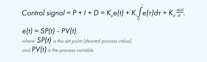
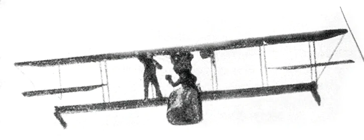
PID controllers have a long history, dating back to the early 20th century. However, their mathematical formulation was developed much later. Today, these controllers are widely used across various industries, from aerospace systems to industrial automation. One of the most challenging aspects of working with PID controllers is tuning them effectively. In this article, we explore the mathematical representations of PID controller gains and how they influence system performance. Proportional–Integral–Derivative (PID) controllers are widely used in many applications today. They are found in motor control systems, flight control units, and power factor correction devices. You can find dozens of these controllers in electric vehicles. PID controllers are also essential in temperature and humidity control systems used in manufacturing, chemical, and pharmaceutical industries. Additionally, they play a key role in power electronics, such as in converters, industrial furnaces, and automated production lines. The PID algorithm uses three components—proportional, integral, and derivative—to calculate the control signal. Each component is multiplied by a gain that determines its influence on the overall output. This allows engineers to fine-tune the controller for specific processes. If you're new to PID controllers, our previous article provides an introduction to the basics. At Integra Sources, our team has extensive experience with PID controllers. We’ve successfully implemented them in numerous projects. If your project requires automation, PID control might be the best solution. Contact us to discuss your needs and get expert guidance. Tuning PID controllers is not always straightforward, even for experienced engineers. While it’s possible to tune them intuitively, there are many nuances involved. In this article, we’ll break down the process and explain the different factors that affect performance. Before diving into the details, let’s start with a brief look at the history of PID controllers. If you search for the first patent on a PID controller, you won’t find one. Back then, the concept wasn’t formalized as a separate device. Instead, engineers referred to the tools that performed similar functions with different names. For example, the device used for automatic course-keeping on ships was called an "automatic helmsman." In reality, it functioned like a basic PID controller. One of the most famous demonstrations of a PID controller was the airplane autopilot. On June 18, 1914, during an exhibition in France, two pilots climbed onto the wings of their plane mid-flight to show that it could fly without manual input. This demonstration captured public attention and led to increased interest in autopilots. As a result, PID controllers gradually replaced manual control. Companies began developing various implementations of the PID mechanism. To avoid patent conflicts, manufacturers had to make modifications. These differences in representation made it difficult for users to switch between systems, creating vendor lock-in and hindering standardization. Interestingly, the mathematical description of the PID controller came more than 10 years after its invention. This means that the technology was initially based on engineering intuition rather than precise mathematical optimization. To understand what makes a well-tuned PID controller, we need to look at transient response performance indicators. These metrics help evaluate how quickly and accurately a system responds to changes. There are several important indicators, including settling time, overshoot, and steady-state error. Let’s examine a hypothetical graph of a transient response to a step input: These indicators help engineers determine whether a PID controller is properly tuned. The goal is to minimize settling time while keeping overshoot and steady-state error within acceptable limits. Understanding how each gain affects the system is crucial for effective tuning. Different representations of these gains can lead to confusion, especially when comparing academic and industrial practices. PID controllers come in different forms, which can affect how they are tuned. The two most common forms are the parallel and series forms. The parallel form is often used in academic settings, while the series form is more popular in practical engineering applications. The choice of form can significantly impact the ease of tuning. For example, the series form tends to be more stable and easier to adjust, making it a preferred option in embedded systems and real-time applications. Adjusting the proportional, integral, and derivative gains can dramatically change the system's behavior. By analyzing the effects of each gain on metrics like settling time and overshoot, engineers can optimize the controller for specific applications. For instance, increasing the proportional gain can speed up the response but may lead to instability. The integral gain helps eliminate steady-state error but can cause overshoot. The derivative gain reduces overshoot but may introduce noise sensitivity. Tuning a PID controller is a complex task that requires both theoretical knowledge and practical experience. With the right approach and understanding of the different forms and representations, engineers can achieve optimal performance in a wide range of applications. Whether you're working on a simple automation system or a complex industrial process, mastering PID control is essential. At Integra Sources, our team of experts is ready to assist you in designing and implementing effective control solutions tailored to your needs. Magnetic Spreader Beam,Adjustable Spreader Bar,Tandemloc Spreader Beam,Adjustable Lifting Beam VOITH CRANE , https://www.voithcraneasia.com
History of PID Controllers
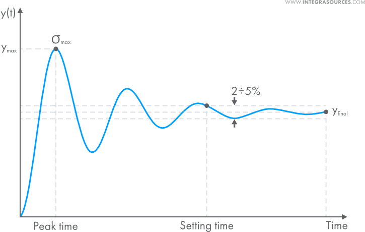
Transient Response Performance Indicators
Representations of PID Gains
Forms of PID Controller
How PID Gains Affect the Transient Response
Conclusion
Mathematical Representations of PID Controller Gains
Contents